Vehicle Routing Problem Optimization

Introduction

High Level Description

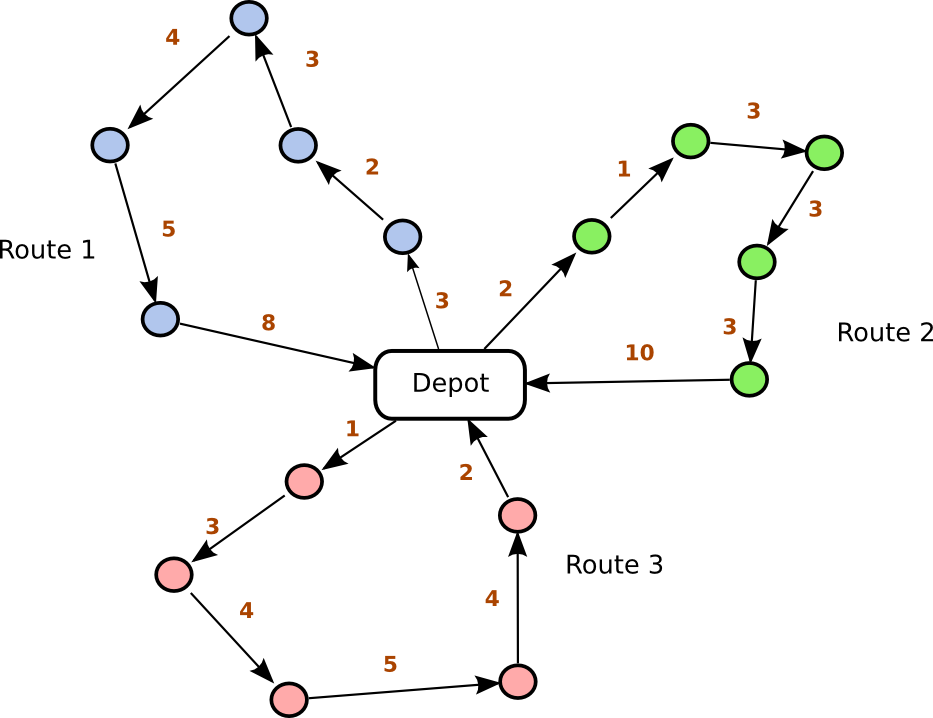
The problem is a combinatorial optimization problem related to graphs. Given a set of vertices which represent physical locations, with a special vertex v0, a central depot, let G = (V, E) be a connected, undirected graph whose weights represents the physical distance between locations. The objective of this problem is given a fleet of vehicles K, what are the most optimal routes for these vehicles to traverse the entire graph, where each route starts and ends at v0. Essentially, the objective is to find an optimal set of cycles that include v0 such that the union of all the cycles is V. The constrained variant of this problem is very similar, but each vertex has a demand associated with it, or a number of packages a vehicle needs to pick up. Additionally, each vehicle has a maximum capacity of packages it can pick up along its route. This problem is a variant of the traveling salesman problem. (more similar to the multi-traveling salesman problem).

This problem was solved using a genetic algorithm and an optimization solver via Python and Google OR Tools.

The motivation for this problem was to study potential algorithms for solving the VRP (Vehicle Routing Problem), especially since there are many real-world applications, such as delivery logistic networks or network traffic routing. The problem seems very interesting and is also graph based, which is a type of problem I wanted to research more.

Figure 1: Example routes for VRP

Challenges

One main challenge to this problem is that this is an NP Hard problem as this problem has a very large solution space. Most algorithms cannot guarantee an optimal solution and only an approximation is typically given. Additionally, since this problem is a graph based problem, the problem formulation itself was a bit difficult, especially deciding on how to encode information. For example, while a decision variable can be used where each variable represents an edge in the graph and takes on the value {0, 1}, this grows in size very quickly for even a small number of cities since the graph is fully connected.

Formulation

Mathematical Model

In this formulation, assume there are two vehicles. This can easily be extended to k vehicles. Let G = (V, E) be a fully connected undirected graph with weights that are the distances between locations. Let v0, v1, …, vn be the set of vertices in the graph where v0 is the depot vertex where every vehicle starts and ends at the depot.

Problem Setup:

• Let A and B represent 2 vehicles.
• Let a = list of vertices A visits and b = list of vertices B visits
• Let p(x, y) = x union y
• Let g(x) be a function that takes in a path and returns the total distance of the path (sum of all edges).
  • For example, g(a) will returns the total distance traveled by vehicle A.
• Let h(x) be a function that takes in a path and returns the total number of packages along a path.
  • For example, h(a) will return the total number of packages along path a.
• Let j(x) be a function that takes in a path and returns 1 if x is a cycle with v0 contained, and 0 otherwise. This function essentially checks if the starting and ending vertex in a path is v0
• Let R be the max capacity for the number of packages a vehicle can pick up. (Assume it’s the same for A and B)

Optimization Formulation

The following is the defined optimization problem without demand/package constraints.

minimize a,b f0(a, b) = max(g(a), g(b))
s.t p(a, b) = {v0, v1, ..., vn}, j(a) = 1, j(b) = 1

The reason the maximum route among vehicles is being minimized is that if simply the maximum total distance in minimized, the solution would just be to traverse the entire graph with 1 vehicle, which is the traveling salesman problem. The routes themselves want to be minimized as deliveries should happen as fast as possible. (more representative of the aims of the VRP, smaller routes = less time) The following constraint can be added to incorporate the aspect of vehicles picking up packages. (capacity vehicle routing problem)

s.t h(a) ≤ R, h(b) ≤ R

This simply states that a given routes’ packages cannot exceed a vehicles capacity.

Numerical Studies

Data Used

For the purposes of this project, 8 locations across campus were chosen as vertices. These locations are: STAMP, Hornbake Library, Business School, McKeldin Library, ESJ, Mowatt Lane Garage, Prince Fredrick Hall, and Skinner building. The vertices are represented with their latitude and longitude and the distances between locations are computed using the Haversine formula. STAMP will be used as the depot location that all routes must start and end at. In addition, for all cases, only 2 vehicles are used. The following are the locations of the 8 buildings.

cord list = [(38.985470, -76.946960), (38.984810, -76.952049), (38.982770, -76.947830), (38.984901,
-76.945221), (38.985780, -76.946930), (38.982208, -76.946953), (38.983080, -76.944970), (38.984480, -
76.941310)]

Demand values for each vertex and the capacity for the vehicles were randomly assigned. The following are the demands and vehicle capacities.

demand list = [0, 2, 4, 8, 3, 1, 5, 1]
vehicle capacities = [12, 12]

Case 1: VRP with no capacity constraints

In this version of the problem, the objective is to minimize the maximum vehicle path. To solve this, a genetic algorithm was implemented in python, and the package mathplotlib was used to plot the graphs. For the genetic algorithm, a gnome, a set of routes, was represented with a list of numbers encoding all route information. An example encoding for the following situation would look like this.

Ex Encoding structure
1: depot
2, 3, 4, 5: customer locations
6, 7: vehicles (however, 6 not included in gnome)
ex encoding
24653
vehicle 7 route: 1 - 2 - 4 - 1
vehicle 6 route: 1 - 5 - 3 - 1

The string starts with the route that vehicle 7 follows until the number 6, where the rest of the string is the route for vehicle 6. With this encoding, the string is only (N-1) + (K-1) characters long and is not dependent on the number of edges.

The fitness function represents the objective function and simply returns the distance of the maximum route in the gnome string. The genetic algorithm utilized a two-point crossover, random mutation, and roulette wheel selection with an ”elite list” where a certain percentage of the population is automatically selected for the next generation. The following resources[4, 5] provided guidance on the programming for this algorithm.

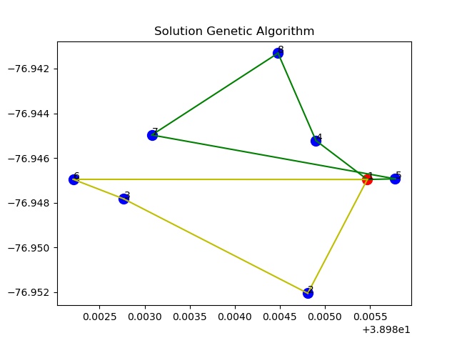
The following is the results for 8 cities defined in the above section using 2 vehicles. The file VRP no constraints genetic algo.py consists of the code for this section.

Figure 2: Solution for VRP without constraints, N = 8, V = 2

Case 2: VRP with capacity constraints

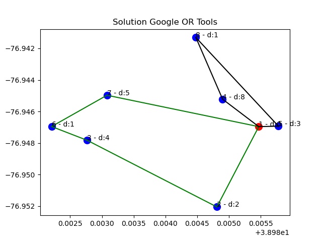
In this variant of the problem, the same 8 cities are used with 2 vehicles. However each vertex has a package number associated with it and each vehicle has a maximum capacity as specified in the section above. To solve this problem, the Google OR tools library was used. (code was referenced from this documentation) This library is capable of solving constrained routing optimization problems. The file VRP API Cons.py consists of the code for this section. The following is the solution produced with this library.

Figure 3: Solution for VRP with constraints, N = 8, V = 2

The maximum route distance for this problem is 1487.13 with the routes [[1, 7, 6, 3, 2, 1], [1, 5, 8, 4, 1]] Note that this distance is larger than the distance without constraints. (due to the extra capacity constrains, reducing the potential solution space)

Discussion and Future Directions

One key observation made was that it is hard to find an optimal solution. Even with a relatively small N, there were many instances where an optimal solution was not found when comparing to the brute force solution. In addition, this problem becomes very computationally extensive as N increases. Additionally, there are many approaches to the same problem, such as using particle swarm vs genetic algorithms.

In the future, I plan to make adjustments to the genetic algorithm to make it more efficient, such as tweaking the selection and crossover process. There are many variants to this algorithm that can impact its efficiency. Additionally, applying the genetic algorithm to the constrained version of the problem would be interesting. Also, running the algorithm for a very large dataset (N > 20) would be an interesting exercise to see how the algorithm performs. Overall, this was an interested problem to study with many real world applications.